🇨🇦 Canadian Grand Prix
Round 5 · 2026 · Circuit Gilles Villeneuve · 5,000 simulations
Updated after Pre-weekend · Sat 23 May, 19:59 UTCYour predictions
Edit site/src/data/predictions/my-predictions.json to enter your own probabilities. Drivers you skip show as "—". Each cell shows your number bold, the model's number muted underneath, and a coloured arrow with the gap in percentage points.
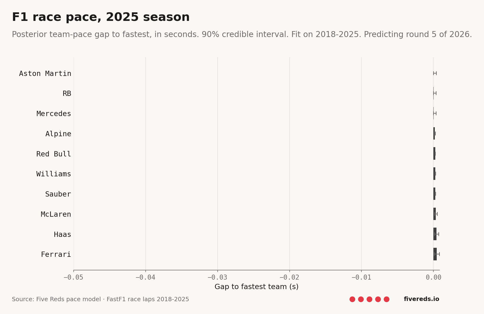
Team pace ladder
Posterior race-pace gap to the fastest team, with 90% credible intervals.
Model accuracy — 2026 baseline
The current model scored against the four completed 2026 races (Australia, China, Japan, Miami). Each race uses a posterior fit only on data before that race's qualifying — leak-free. This is the baseline to beat with model improvements.
favourite actually won
who actually podium'd (avg)
(baseline 0.185)
Pole prediction: Bayesian vs simple position-based model
| Model | Log-loss | Baseline | Favourite hit | Verdict |
|---|---|---|---|---|
| Bayesian (current quali model) | 1.319 | 0.185 | — | worse than baseline |
| Simple position-based (new) | 0.198 | 0.185 | 3/4 | worse than baseline |
Per-market scores
| Market | N | Log-loss | Baseline | Brier | ECE | Verdict |
|---|---|---|---|---|---|---|
| Win | 88 | 0.268 | 0.185 | 0.064 | 0.083 | worse than baseline |
| Podium | 88 | 0.298 | 0.398 | 0.108 | 0.086 | beats baseline |
| Points | 88 | 0.701 | 0.689 | 0.228 | 0.143 | worse than baseline |
| Pole | 88 | 1.319 | 0.185 | 0.068 | 0.091 | worse than baseline |
| Finish | 88 | 0.534 | 0.537 | 0.173 | 0.067 | beats baseline |
| Team H2H | 219 | 0.780 | 0.693 | 0.249 | 0.207 | worse than baseline |
Per-race breakdown
Australian Grand Prix
Actual
- Winner
- Russell
- Pole
- Russell
- Podium
- AntonelliLeclercRussell
- DNFs
- AlonsoBottasHadjarHülkenbergPiastriStroll
Model's pre-race top 5 to win
| # | Driver | P(win) | Result |
|---|---|---|---|
| 1 | Norris | 46.4% | Finished |
| 2 | Piastri | 44.4% | DNF |
| 3 | Hamilton | 3.1% | Finished |
| 4 | Leclerc | 2.8% | Podium |
| 5 | Antonelli | 0.9% | Podium |
Simple model's pre-race top 5 to pole
| # | Driver | P(pole) | Result |
|---|---|---|---|
| 1 | Russell | 60.4% | Pole |
| 2 | Norris | 20.6% | — |
| 3 | Verstappen | 10.3% | — |
| 4 | Piastri | 8.6% | — |
| 5 | Alonso | 0.0% | — |
Chinese Grand Prix
Actual
- Winner
- Antonelli
- Pole
- Antonelli
- Podium
- AntonelliHamiltonRussell
- DNFs
- AlbonAlonsoBortoletoNorrisPiastriStrollVerstappen
Model's pre-race top 5 to win
| # | Driver | P(win) | Result |
|---|---|---|---|
| 1 | Piastri | 46.3% | DNF |
| 2 | Norris | 46.1% | DNF |
| 3 | Leclerc | 2.4% | Finished |
| 4 | Hamilton | 2.3% | Podium |
| 5 | Russell | 1.0% | Podium |
Simple model's pre-race top 5 to pole
| # | Driver | P(pole) | Result |
|---|---|---|---|
| 1 | Verstappen | 95.0% | — |
| 2 | Russell | 2.3% | — |
| 3 | Piastri | 1.6% | — |
| 4 | Hadjar | 0.8% | — |
| 5 | Norris | 0.3% | — |
Japanese Grand Prix
Actual
- Winner
- Antonelli
- Pole
- Antonelli
- Podium
- AntonelliLeclercPiastri
- DNFs
- BearmanStroll
Model's pre-race top 5 to win
| # | Driver | P(win) | Result |
|---|---|---|---|
| 1 | Norris | 47.8% | Finished |
| 2 | Piastri | 43.9% | Podium |
| 3 | Leclerc | 3.0% | Podium |
| 4 | Hamilton | 2.3% | Finished |
| 5 | Antonelli | 1.1% | Won |
Simple model's pre-race top 5 to pole
| # | Driver | P(pole) | Result |
|---|---|---|---|
| 1 | Russell | 37.6% | — |
| 2 | Leclerc | 24.2% | — |
| 3 | Verstappen | 20.7% | — |
| 4 | Antonelli | 11.9% | Pole |
| 5 | Piastri | 3.2% | — |
Miami Grand Prix
Actual
- Winner
- Antonelli
- Pole
- Antonelli
- Podium
- AntonelliNorrisPiastri
- DNFs
- GaslyHadjarHülkenbergLawson
Model's pre-race top 5 to win
| # | Driver | P(win) | Result |
|---|---|---|---|
| 1 | Piastri | 47.8% | Podium |
| 2 | Norris | 44.0% | Podium |
| 3 | Leclerc | 2.6% | Finished |
| 4 | Hamilton | 2.5% | Finished |
| 5 | Antonelli | 1.2% | Won |
Simple model's pre-race top 5 to pole
| # | Driver | P(pole) | Result |
|---|---|---|---|
| 1 | Antonelli | 56.0% | Pole |
| 2 | Russell | 20.1% | — |
| 3 | Leclerc | 17.9% | — |
| 4 | Verstappen | 3.4% | — |
| 5 | Piastri | 1.2% | — |
Canadian Grand Prix
Actual
- Winner
- —
- Pole
- —
- Podium
- DNFs
- none
Model's pre-race top 5 to win
| # | Driver | P(win) | Result |
|---|
Simple model's pre-race top 5 to pole
| # | Driver | P(pole) | Result |
|---|---|---|---|
| 1 | Russell | 49.9% | — |
| 2 | Antonelli | 26.8% | — |
| 3 | Verstappen | 12.1% | — |
| 4 | Piastri | 6.4% | — |
| 5 | Leclerc | 2.7% | — |
Source · 2026 walk-forward backtest · Method SVI · Refit cadence weekend · 5,000 simulations per race · Each race scored on a posterior fit only on data prior to that race's qualifying.
Inside the model
The exact numbers the simulator drew from. Every probability on this page is downstream of the trajectories and hyperparameters below.
AR(1) team-pace evolution
Each line is one team's β_team_year across every season in the training window. The curve is the random walk β[s, t] = β[s-1, t] + ε that the model fit. Lower lines = faster cars. The big move on the right edge is the 2026 step — what 2026 lap data has done to each team's posterior. Hover a team in the legend to isolate it.
Fitted hyperparameters
What the model has learned about its own structure. The "posterior" column is the 90% credible interval after fitting on 2018-2026 data; compare it to the "prior" column to see whether the data moved the model's belief.
Pace model
| Symbol | What it is | Prior | Posterior (90% CI) |
|---|---|---|---|
μ_circuit | Population log-lap-time intercept | Normal(log 85, 0.5) | 2.858[2.857, 2.859] |
σ_team_init | Spread of teams in year-1 baseline (log-s) | HalfNormal(0.2) | 0.7035[0.7003, 0.7073] |
σ_year_step | AR(1) year-to-year drift (log-s) | HalfNormal(0.05) | 0.0659[0.0657, 0.0661] |
σ_circuit | Spread of per-race base lap times | HalfNormal(0.5) | 1.062[1.061, 1.063] |
σ_compound | Soft/medium/hard offset spread | HalfNormal(0.02) | 0.0175[0.0163, 0.0186] |
φ_fuel | Fuel-burn slope per fuel-fraction | Normal(-0.012, 0.01) | -0.0369[-0.0390, -0.0350] |
ψ_tyre | Tyre-wear slope per lap of age | Normal(0.0006, 0.0005) | 0.0003[0.0001, 0.0005] |
σ (lap noise) | Within-stint lap-to-lap residual | HalfNormal(0.05) | 0.0210[0.0199, 0.0223] |
Qualifying model
| Symbol | What it is | Prior | Posterior (90% CI) |
|---|---|---|---|
σ_team_init | Spread of teams in year-1 baseline (log-s) | HalfNormal(0.2) | 0.0206[0.0194, 0.0221] |
σ_year_step | AR(1) year-to-year drift | HalfNormal(0.05) | 0.0013[0.0011, 0.0014] |
σ_circuit | Spread of per-race quali baselines | HalfNormal(0.5) | 0.7491[0.7488, 0.7494] |
σ_segment | Q1/Q2/Q3 track-evolution offset | HalfNormal(0.05) | 0.0799[0.0795, 0.0802] |
Reliability model
| Symbol | What it is | Prior | Posterior (90% CI) |
|---|---|---|---|
μ_dnf | Population logit DNF rate | Normal(logit 0.15, 0.5) | -1.766[-1.830, -1.692] |
σ_team_init | Spread of teams in year-1 DNF baseline | HalfNormal(0.5) | 0.1938[0.1338, 0.2662] |
σ_year_step | AR(1) year-to-year drift in DNF rate | HalfNormal(0.2) | 0.0440[0.0190, 0.0870] |
σ_circuit | Per-circuit DNF-rate spread (logit) | HalfNormal(0.5) | 0.1519[0.0938, 0.2248] |
How these predictions are made
The number in each cell is the fraction of 10,000 simulated races where that driver hit that result. The simulator draws from three Bayesian models fit on every clean-air race lap from 2018 to today.
The rest of this page is a long, technical explanation of the model. If you just want to read the table and move on, you can stop here.
What each column means
Pole
Probability of starting first on the grid. Computed from the qualifying model only — single-lap pace, fresh tyres, low fuel. The race result has no effect on this column.
Finish
Probability of being classified at the chequered flag (i.e. not retiring). Computed from the reliability model only — a logistic regression on whether each (team, circuit) combination historically DNFs.
Points
Probability of finishing P1–P10. From the race simulator — combines pace + reliability across 10,000 sims.
Podium
Probability of finishing P1–P3. Same simulator, stricter threshold.
Win
Probability of finishing P1. Same simulator, strictest threshold.
Exp.
Mean finish position across 10,000 sims (DNFs treated as last). A summary number — sortable but not a probability.
Three models, five markets — why the count differs
The three models capture three independent statistical objects you can fit from F1 data: race-stint pace, single-lap pace, and finish/DNF. Of the five markets, Pole comes from the qualifying model alone, Finish from the reliability model alone, and Win / Podium / Points are not separate predictions — they're the same race-outcome distribution counted at finish-position thresholds of 1, 3, and 10. Counting from a single simulation guarantees P(win) ≤ P(podium) ≤ P(points) automatically.
The pace model — full specification
Fits clean-air race lap times. ~135,000 rows, one per (session, driver, lap) for every clean lap 2018–2026. A clean lap is IsAccurate + green track + not pit-in/out + not stint-warmup + not stint-final.
log(lap_time_s)  =  β_team_year[s, t]
                  +  γ_circuit[s, r]
                  +  δ_compound[c]
                  +  φ_fuel  · fuel_lap_norm
                  +  ψ_tyre  · tyre_age
                  +  ε
ε ~ Normal(0, σ) | Term | Prior | What it is |
|---|---|---|
β_team_year[s, t] | β[s_0, t] ~ Normal(0, σ_team_init)β[s, t] = β[s-1, t] + εε ~ Normal(0, σ_year_step)σ_team_init ~ HalfNormal(0.2)σ_year_step ~ HalfNormal(0.05)+ sum-to-zero across teams per year | AR(1) random walk per team. Last season's effect is the prior mean for this season's, with σ_year_step controlling year-to-year drift. Strong recent form gets absorbed; weak 2026 evidence falls back to 2025 form, not zero. Sum-to-zero across teams within each year fixes an identifiability ambiguity with μ_circuit: only relative team gaps live in β; absolute level lives in μ.
|
γ_circuit[s, r] | Normal(μ_circuit, σ_circuit)μ_circuit ~ Normal(log 85, 0.5)σ_circuit ~ HalfNormal(0.5) | Per-(season, round) base lap time. μ_circuit is the population mean (~85s, the historical median lap). Each (season, round) gets its own cell — round 1 in 2018 (Australia) and round 1 in 2020 (Austria) are different races. |
δ_compound[c] | Normal(0, σ_compound)σ_compound ~ HalfNormal(0.02) | Soft/medium/hard offset. Tight prior because compound deltas are typically 0.5–1s — small in log terms. |
φ_fuel | Normal(-0.012, 0.01) | Fuel-burn slope. Cars get faster as they get lighter. The prior centres on -1.2% per fuel-fraction (informed by physics), with a tight standard deviation. |
ψ_tyre | Normal(0.0006, 0.0005) | Tyre-wear slope. Lap times grow at ~0.06% per lap of tyre age. |
σ (lap noise) | HalfNormal(0.05) | Within-(team, race, compound) lap-to-lap noise. Includes driver skill (no α_driver in v1), traffic, weather variation. The thing the team-pace prior had to compete with. |
Non-centred reparameterisation
Hierarchical Bayesian models fit better when you decouple the scale parameter from the unit-effects. Internally the model stores z_team_year ~ Normal(0, 1) and constructs β_team_year = σ_team_year × z_team_year. NUTS samples through this much more cleanly than the centred form, which is why every coefficient in the model has the same trick.
The qualifying model
Fits a single observation per (session, driver) — the fastest single lap that driver set across Q1/Q2/Q3.
log(best_lap_s)  =  β_team_year[s, t]
                  +  γ_circuit[s, r]
                  +  δ_segment[Q1 / Q2 / Q3]
                  +  ε
        ε  ~  Normal(0, σ)
Same priors as the pace model for β_team_year, γ_circuit, and σ. No fuel or tyre slope — quali is single-lap, low-fuel, fresh tyres. δ_segment captures track evolution: the same driver's identical effort in Q1 vs Q3 logs different times because the track rubbers in. Without this, drivers who only progressed to Q1 would look slower than they are.
The reliability model
Bernoulli on whether each (driver, race) ended in DNF. One row per driver per race; ~500 rows per season × 8 seasons.
logit(P_DNF)  =  μ_dnf
              +  β_team_year[s, t]
              +  γ_circuit[circuit_id]
is_dnf  ~  Bernoulli(sigmoid(logit_P_DNF))
Different from pace/quali in three ways:
- Likelihood family. Bernoulli with a logit link, not Gaussian on log-time. Same hierarchical-Normal priors on the coefficients, applied through the logit transform.
- Circuit identifier. Uses the canonical Ergast
circuit_idpooled across years, not(season, round). Monaco is persistently accident-prone in 2018 and 2024 alike — pooling concentrates that signal. With ~22 races/season × 20 drivers = 440 rows/season per circuit, splitting by(season, round)would dilute it. - Population baseline.
μ_dnf ~ Normal(-2, 1)centres the prior on a ~12% DNF rate (sigmoid of -2), close to the long-run F1 average. Per-team and per-circuit effects shift this up or down on the logit scale.
How we fit the posteriors
Both NUTS (No-U-Turn Sampler, gradient-based MCMC) and SVI (Stochastic Variational Inference, fast approximation) are supported. NUTS is the default for production runs — slower but exact, sampling roughly 500 warmup + 500 posterior draws per model. SVI uses an AutoNormal guide and is used during development for fit-window experimentation. Both produce the same shape of output: a sample-by-coefficient array that the simulator draws from.
Posteriors are content-addressed by their inputs hash (since, until, method, n_rows, n_drivers, n_teams, num_samples) and cached on disk, so refitting on the same data is a no-op. That's how the per-session workflow stays cheap: the heavy NUTS fit runs weekly, intra-weekend session updates reuse the cached posterior.
Leak-free temporal cutoff
Every fit uses an as_of timestamp that defaults to one second before the target race's qualifying session. Training data filters to laps and results that finished before that timestamp. This is what makes backtesting honest: the 2024 Imola prediction sees only the data the model would have had at the moment of qualifying, not the race outcome it's trying to predict.
The simulator — step by step
- Draw one joint sample from the three posteriors (one realisation of all coefficients).
- For each driver, compute predicted log-lap-time as
β_team_year[2026, their team] + γ_circuit[2026 R5]. (When the target race's circuit cell isn't in the encoder — typical for upcoming rounds — fall back toμ_circuit.) - For each of the 60-ish laps, draw a multiplicative noise term
(1 + σ × Normal(0, 1))and apply it to the driver's lap time. - Sum the laps → race time.
- Roll a DNF outcome from
Bernoulli(sigmoid(μ_dnf + β_rel + γ_rel)). - Compute quali time the same way as race lap time but using the quali model's posteriors → quali rank.
- Sort drivers by race time. DNFs go to position 0 (sentinel).
- Record finish position, quali rank, race time, DNF flag for each driver.
- Repeat 10,000 times. Aggregate fractions per market.
Identifiability and design choices
A few non-obvious model decisions, and why:
- No driver effect (α_driver). Driver and team are colinear in F1 data — drivers move teams rarely, so a per-driver / per-team coefficient pair fits non-uniquely. With weak priors the fit collapses on whichever side gets first dibs and rankings come out garbled. With tight priors it doesn't recover. The fix is a separate residual model fit on within-team-year teammate gaps, where the colinearity disappears (you're comparing two drivers in the same car). That's planned for v2.
- Per-(season, round) circuit cells, not per-circuit. The same physical track is a different race in different years (regulations change, tarmac is resurfaced, weather differs). Pooling across years would smear those changes. The reliability model is the exception — DNF rates are dominated by track geometry, which is stable.
- AR(1) cross-year structure for β_team_year (added 2026-05-08). Each team's per-year effect is now a Gaussian random walk across seasons:
β[s, t] = β[s-1, t] + εwithε ~ Normal(0, σ_year_step). Last season is the prior mean for this season, so strong recent form gets absorbed without having to overcome an at-zero prior. Sum-to-zero per year removes the identifiability ambiguity withμ_circuit. - Pace model has no
α_driver, but lap noiseσabsorbs driver-skill variance. This means the lap noise is wider than it should be, which is part of why team gaps had to fight uphill against the data.
What's NOT in the model
- No driver effect. Drivers in the same (season, team) predict identically. Verstappen and his teammate get the same race-pace forecast. The gap you sometimes see between teammates in this table is pure Monte Carlo noise.
- No track-position effect. The race simulator does not use grid position to determine race outcome. A car predicted to be slowest in qualifying but fastest in race trim would still "win" the simulation. Monaco predictions in particular will look wrong because real Monaco is ~80% determined by qualifying.
- Year-to-year drift prior is a single parameter.
σ_year_stepis shared across all teams. In reality some teams' form is stable (McLaren 2024-2026), others volatile (Williams across regulation changes). Per-team year-step variance is a v3 enhancement. - No tyre-strategy model. Pit-stop timing, undercut/overcut effects, 1-stop vs 2-stop choices are not modelled. The pace model captures average stint pace; the strategic decisions made on top of that aren't.
- No weather conditions. Wet vs dry races have completely different pace orderings, and the model treats them identically.
- No live form features — practice times, sprint results, mid-session tyre data, free-practice fuel-corrected pace. These exist in the data but don't feed the model.
The page reflects engine output verbatim. Every number above came out of the simulator, not editorial judgement. If a column looks wrong, the fix lives in the model, not in the display.
Source · Five Reds Engine · Method SVI · Fit window 2018–2026